2. Application of the risk assessment methodology

2.1 What is risk?

Risk is the likelihood of a hazard occurring, whereas a hazard is something that has the potential to cause harm, based on exposure and vulnerability to that hazard.

In assessing fire risk, the fire represents the hazard, and the likelihood of fire is examined as a function of past fire history (incident data from FRV and the CFA). Response time affects the level of exposure to the hazard. Casualties result from both exposure and vulnerability to the fire and may be viewed as an impact or consequence of the fire.

In addition to fire incidents, the Panel has also considered motor vehicle accidents (MVAs) in the assessment of risk due to the potential for the ignition of fuel.

2.2 Assessment of fire risk

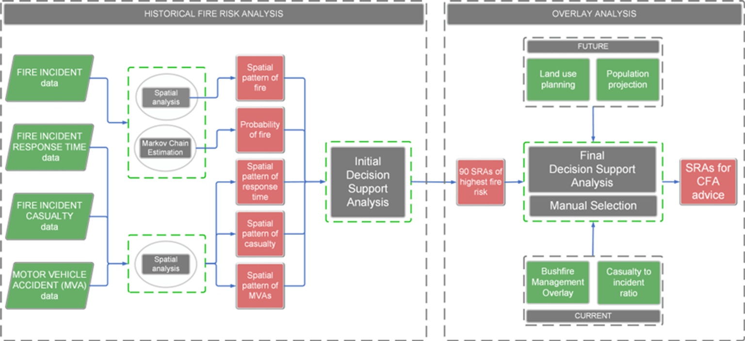
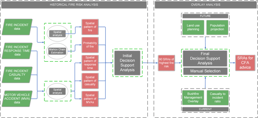
Fire risk is assessed using a combination of techniques. An overview of the fire risk assessment methodology is presented in Figure 1.

Fire-related incidents, casualties, associated response times, and MVA data are examined via various spatial and statistical techniques at the SA1 scale.

Fire risk was also modelled using a probabilistic technique to explore the likelihood of fire over the spatial extent.

The output of these techniques was reviewed for accuracy and subsequently collated in a single feature class layer and stored in geodatabase file for input into the initial decision support analysis (DSA).

This representation of fire risk at the SA1 scale is then spatially attributed to individual station response areas (SRAs). Other pertinent information is attributed to the SRAs, including bushfire, planning, and projected population information.

Specific incident-related data (casualty to incident ratios) is also calculated for each SRA. Review of this data and a final application of the DSA produced the Panel’s determination, which is a final listing of SRAs for which CFA advice is required.

2.3 Changes in fire risk

Considering the definition of a change in fire risk as defined in section 3(1) of the Act, this work has established the fire risk for SRAs. The examination of change in fire risk considered datasets that represent a demand on each SRA (identified using Bushfire Management Overlay [BMO] and casualty to incident ratios), as well as the location of SRAs in terms of future demand (identified using Victorian Planning Authority [VPA] planning and population projections).

2.4 Spatial analysis of fire risk

Understanding the risk of fire associated with historical fire incidents is critical for effective placement of the fire district boundaries. Historical incidents of fire, MVAs, casualty and Service Delivery Standard (SDS) failure associated with fire have been spatially assessed using a range of spatial and statistical techniques, as outlined in the following sections.

2.4.1 Bivariate mapping

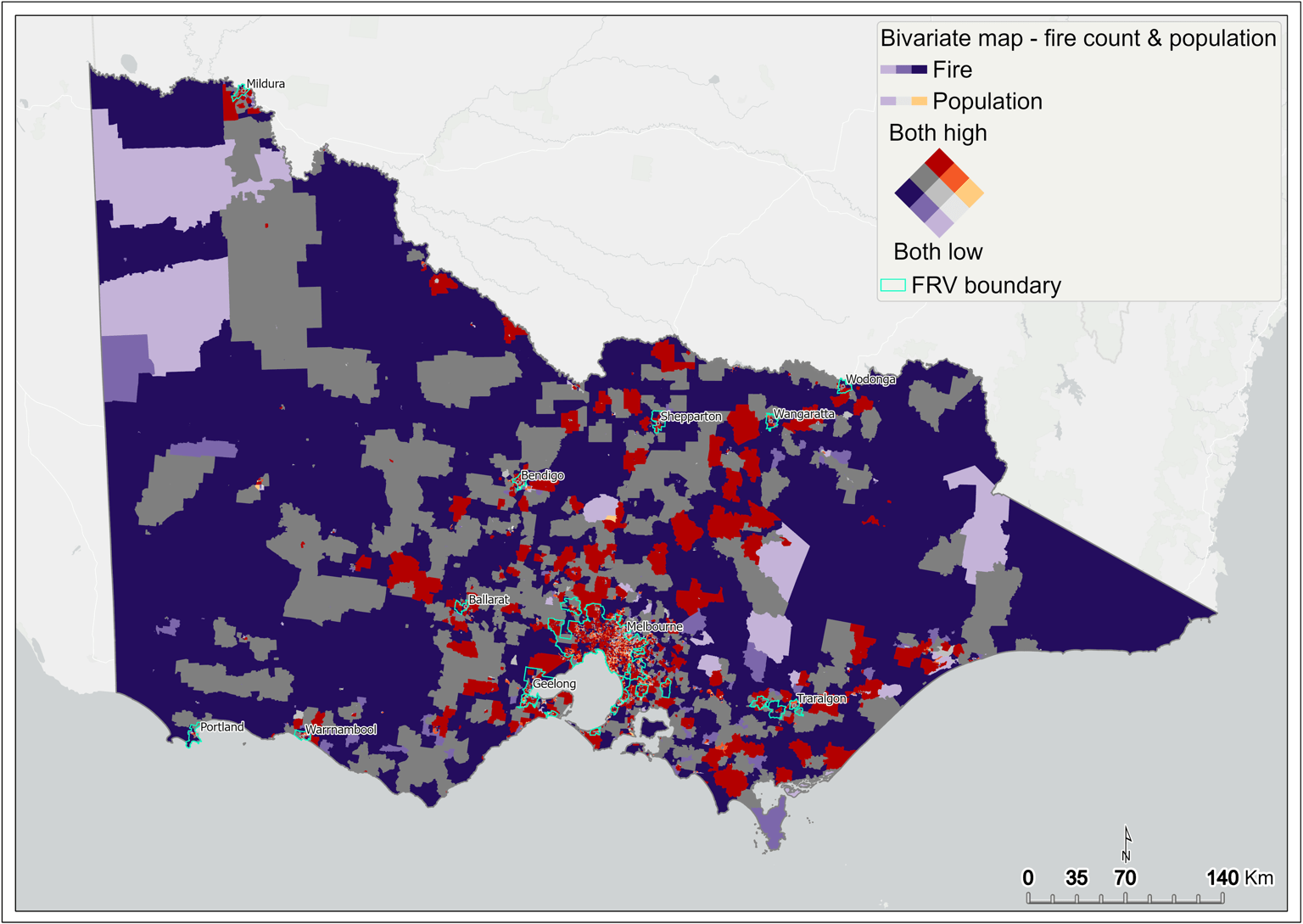
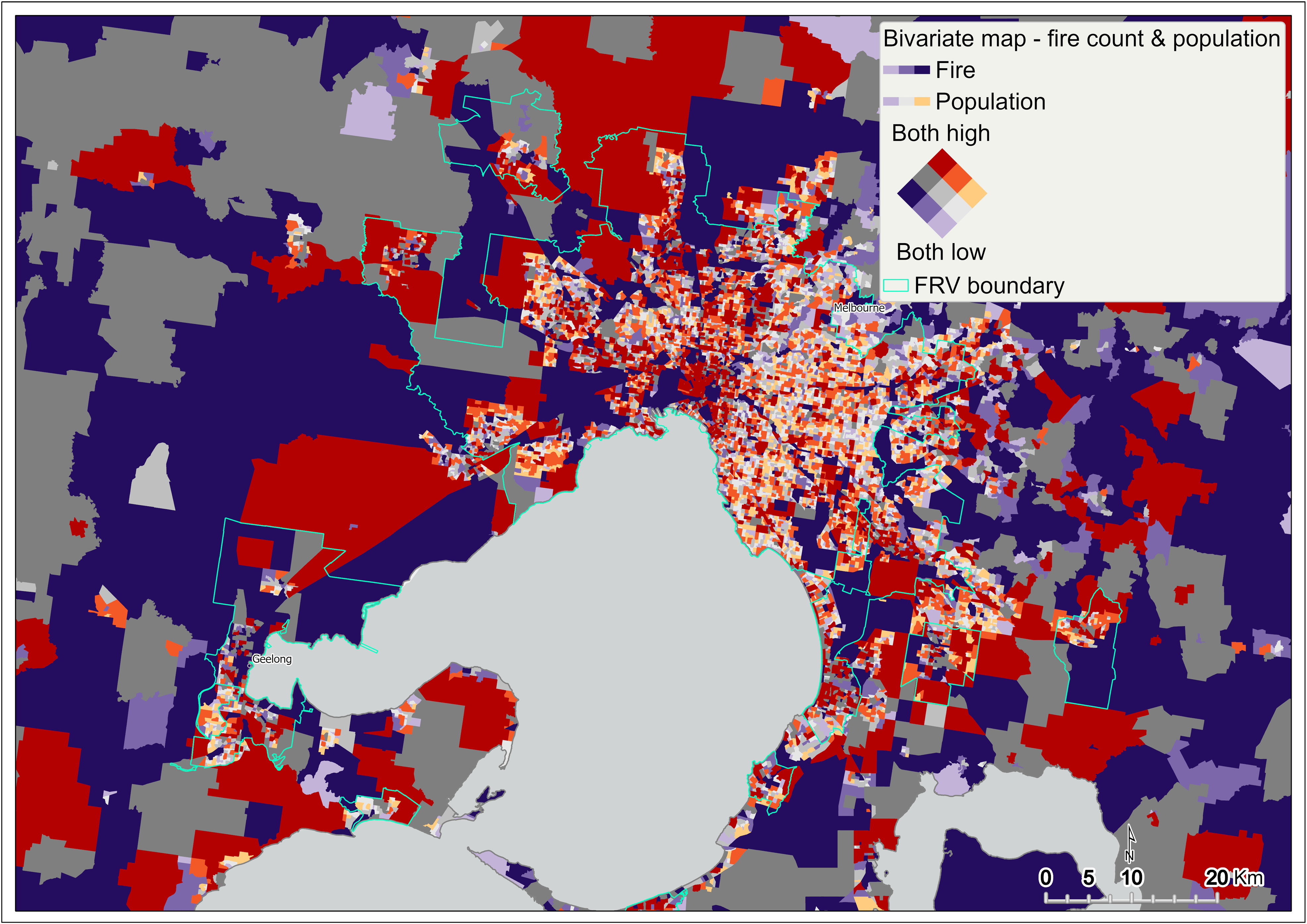
Bivariate² mapping is computed by mapping the fire count and total population across all SA1s in Victoria. It identifies areas that have both high fire count and population (Figure 2, Figure 3).

This analysis has two aims:

• to understand the spatial relationship between fire count and underlying population in Victoria
• to capture SA1 areas containing both high fire count and high population count in Victoria, to compute fire rate mapping on these SA1s, and to use this result as one of the components in the DSA. This method overcomes the disparity between the population in regional Victoria and metropolitan Melbourne when calculating the fire rate.

2.4.2 Fire rate

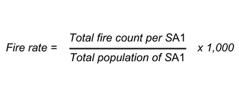
Drawing on the bivariate mapping output (only for SA1s containing high population and fire count), fire rate is computed by dividing the total fire counts by the total population of the SA1 and multiplied by 1,000.

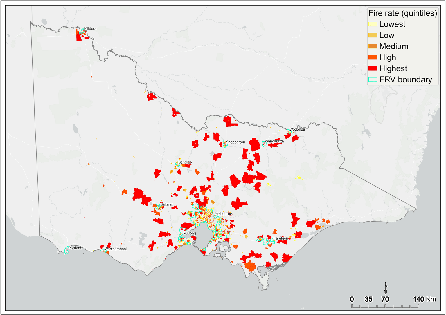
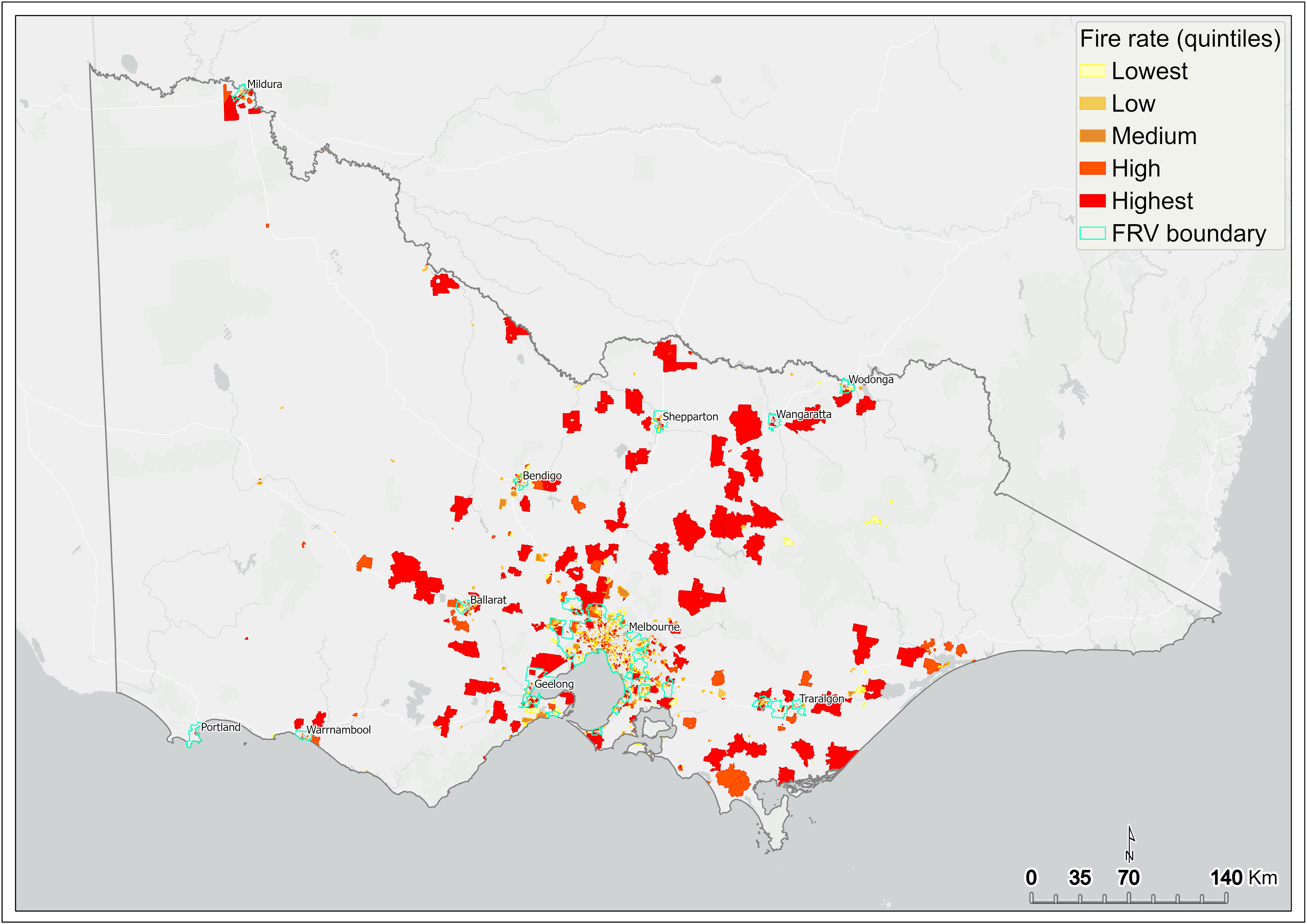
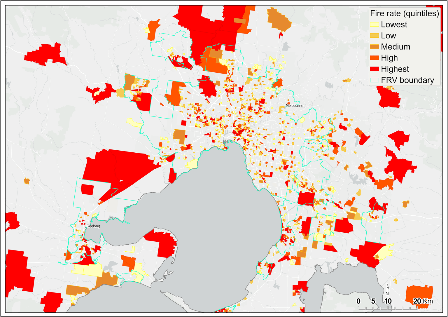
This analysis revealed the fire rate as being highest in SA1s scattered across metropolitan Melbourne, as well as in the regions extending to the New South Wales border, central Gippsland, and the Central Highlands (Figure 4, Figure 5). The subsequent fire rate output was input to the initial DSA.

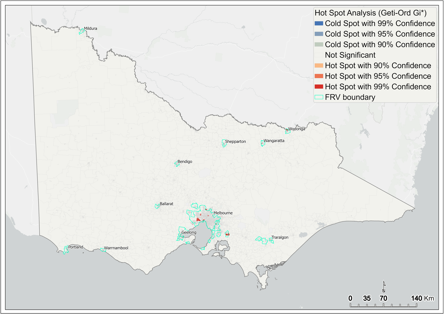
2.4.3 Hot spot analysis

Hot spot analysis, also known as Getis-Ord Gi* (G-I-star) statistics, identifies locations of statistically significant³ clusters of high values (hot spots) and low values (cold spots). This work focused on the statistically significant hot spots, using the fire rate (per 1,000 people) across SA1 of Victoria.

The hot spot analysis returns a z-score and a p-value for each polygon.

• The p-value is a probability.
• Z-scores are standard deviations.
• A high z-score and a low p-value for a feature indicates a significant hot spot.
• The higher the z-score (or lower if negative), the more intense the clustering.
  For statistically significant positive z-scores, the larger the z-score, the more intense the clustering of high values (hot spot).
• A z-score near zero means no spatial clustering.

A key step in the spatial hot spot analysis is selecting an appropriate distance threshold (or band) for analysis. For this, an incremental spatial autocorrelation test was used. Drawing on the Global Moran’s I Index value (0.032533), an appropriate distance threshold of 1,500 m was selected using an associated zscore of 9.475181 and a p-value of 0.000000.

To validate the results obtained from the hot spot analysis, a spatial autocorrelation test was used to determine whether the pattern observed from the hot spot analysis could be the result of random chance. The spatial autocorrelation report, which has a Moran′s Index value of 0.397936, identified significant positive clustering of fires at a global level across the study area (z = 115.417437, p = 0.000000).

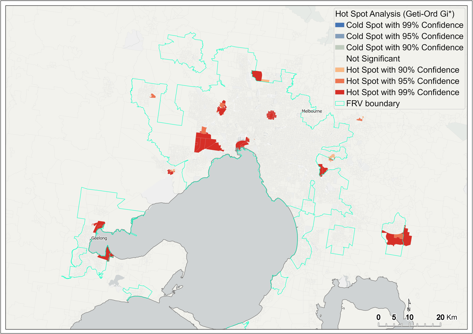
The output of the analysis shows that features of high values cluster spatially. Figure 6 shows hot spots with 99 per cent confidence interval in red; these are mainly concentrated in and around metropolitan Melbourne. On Melbourne’s outskirts, significant hot spots are seen in Geelong and Pakenham (Figure 7). In the regions, significant hot spots are only seen in the north of the state, around Wangaratta and Wodonga (Figure 6).

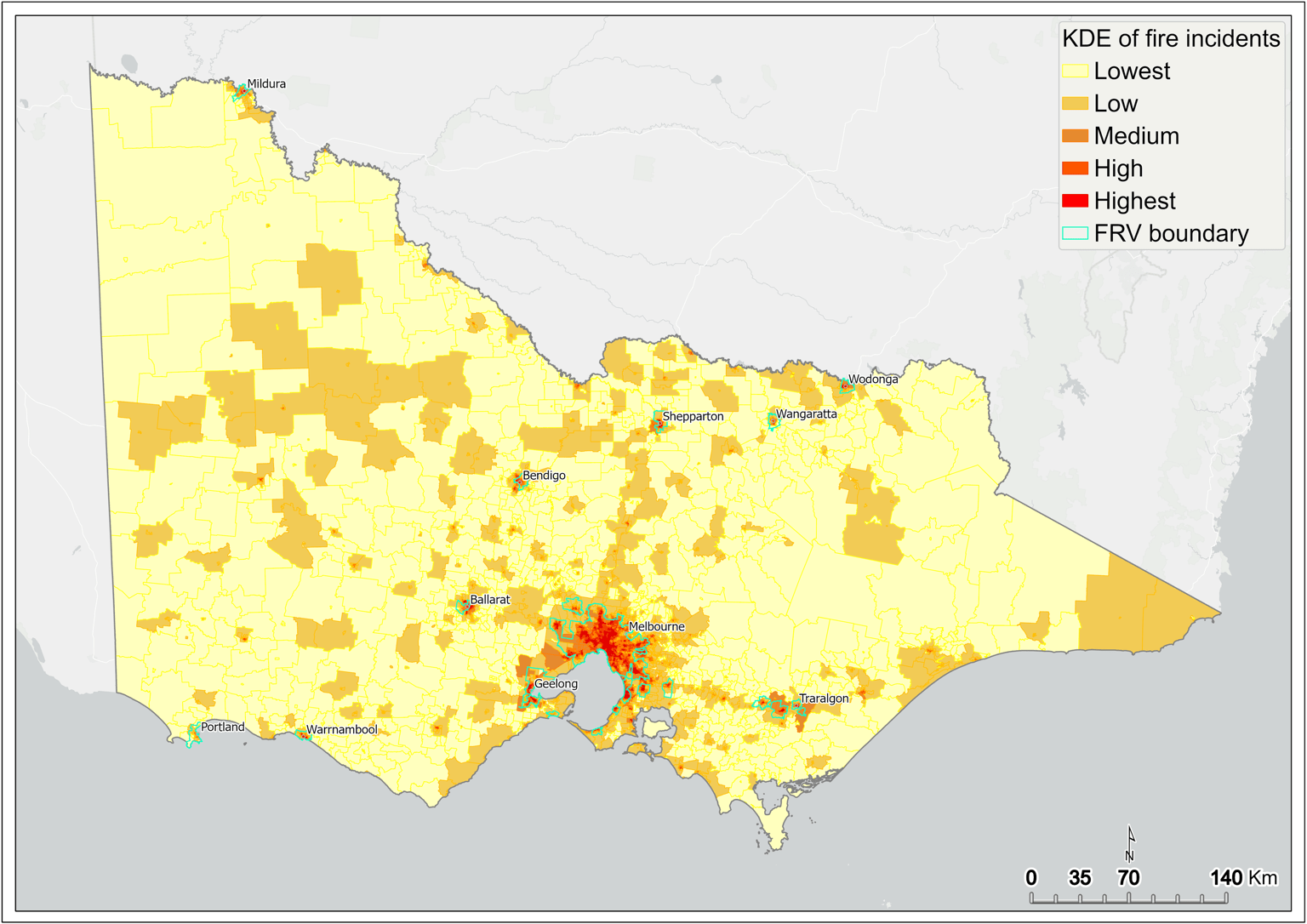
2.4.4 Kernel density estimation

In this review, the kernel density estimation (KDE) technique was used to highlight the spatial variability of both fire incidents and MVAs across Victoria. The KDE map identifies areas exhibiting high concentrations of these incidents, also known as ‘hot spots’ in contrast to those displaying lower incidence levels.

While the previous techniques (fire rate and hot spot analysis) are constrained by using SA1 boundaries, KDE analysis is computed to identify areas exhibiting high incident intensity independent of any geographical boundary. The raster output from the KDE (classified values) analysis is converted into vector format (using a common scale, SA1) to facilitate input into the initial DSA.

A key factor in the use of KDE is the selection of an appropriate distance band (bandwidth or threshold). This bandwidth determines the search radius that the KDE technique employs. A larger bandwidth produces a smoother, more generalised density output, while a very small one produces a more detailed output. After testing a range of bandwidths, 1,000 m was selected to compute the KDE of fire incidents and MVAs.

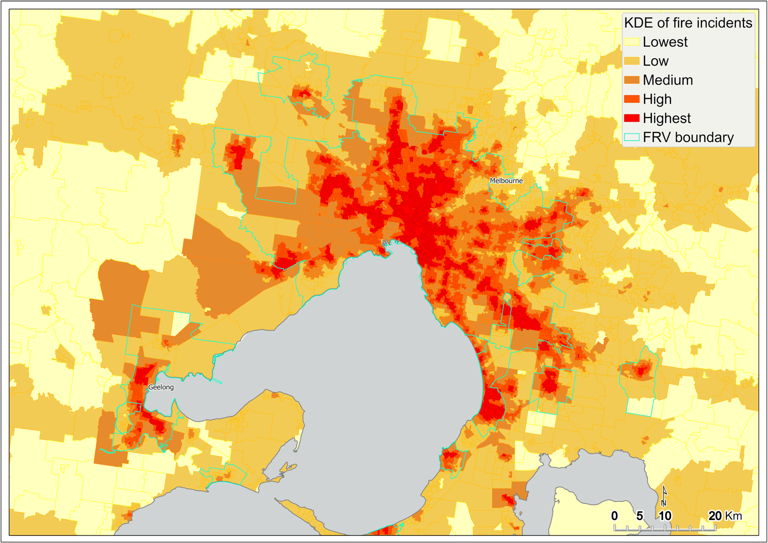
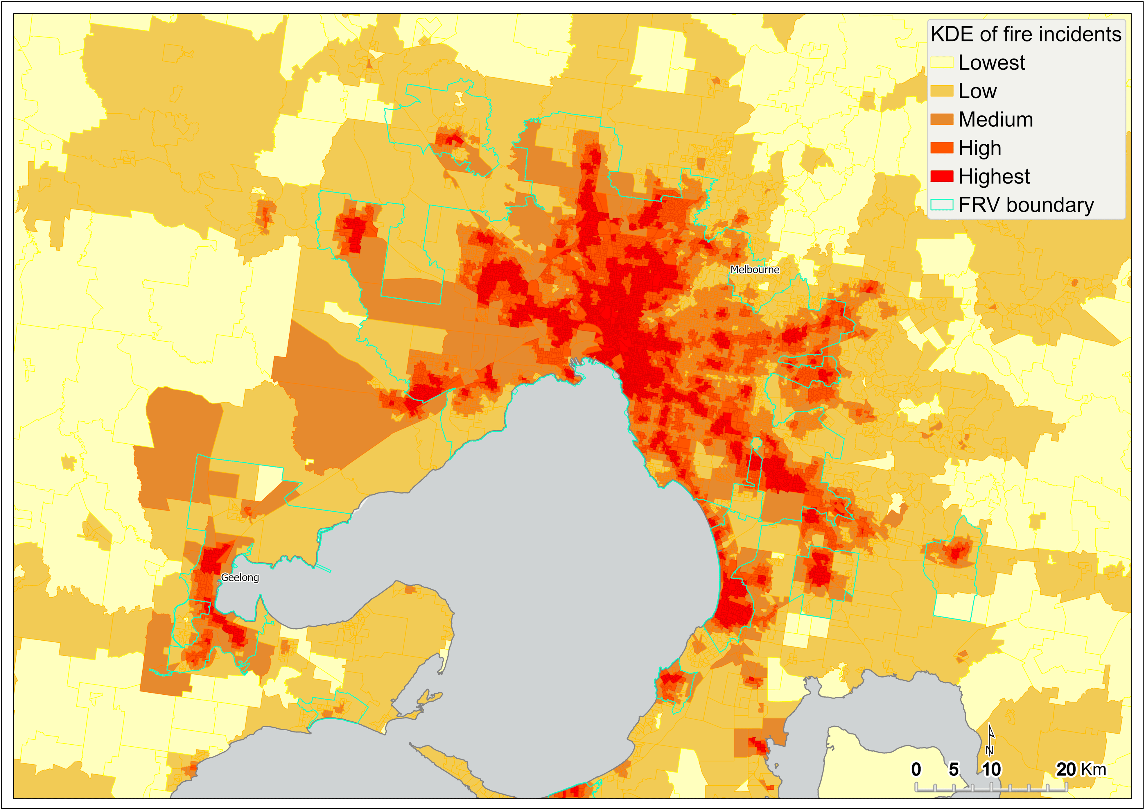
Figure 8 shows the KDE of fire incidents captured at the SA1 scale across Victoria. Results show that the intensity of fire is highest in Melbourne’s CBD and many of the inner-city suburbs (Figure 9). Intensity is also high in many of the larger regional centres, such as Ballarat, Bendigo, Geelong, Mildura, Albury, and Shepparton (Figure 8).

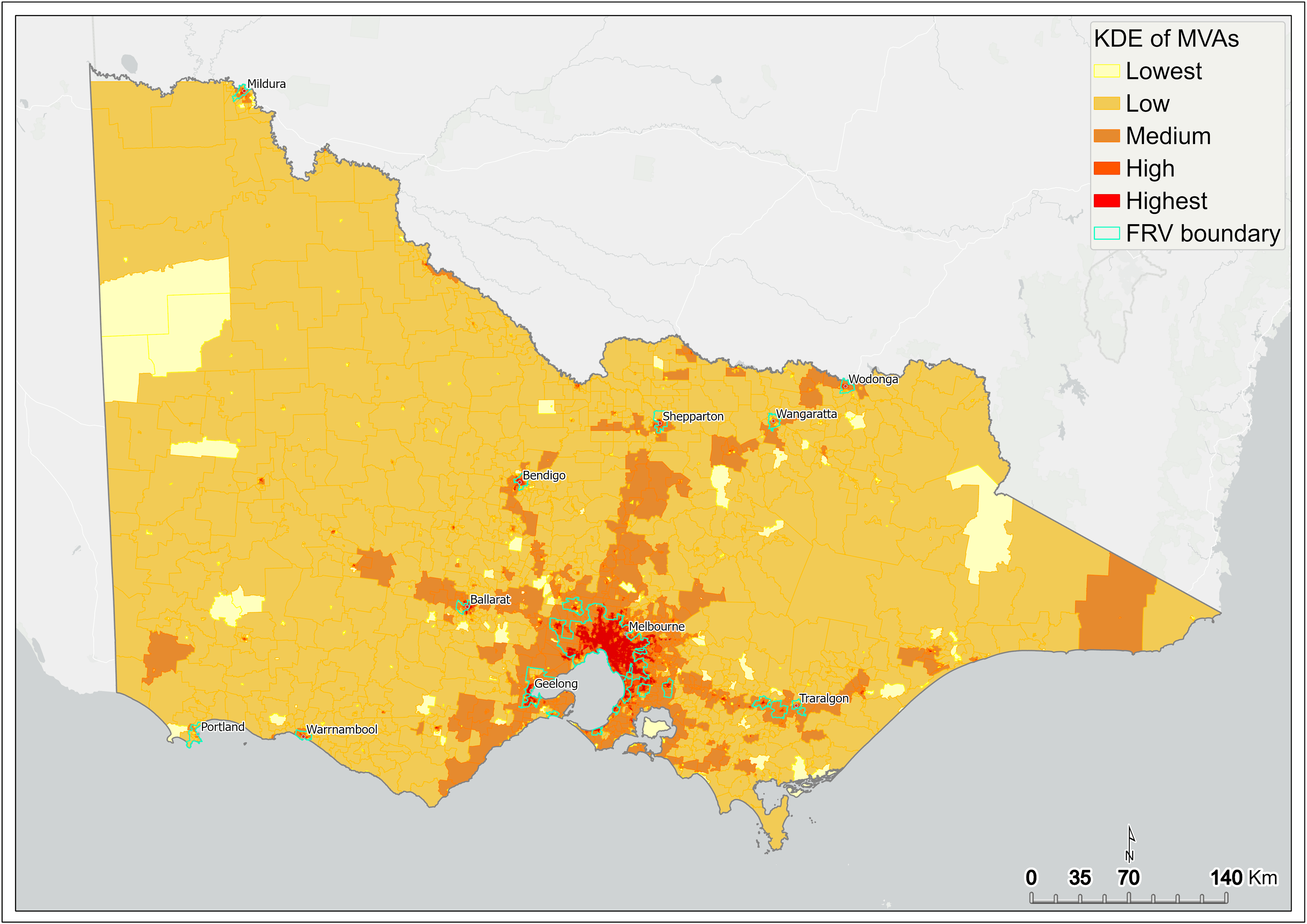
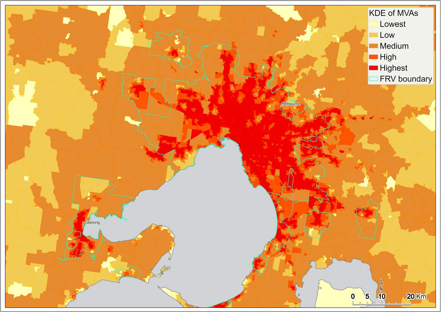
A similar pattern is exhibited by KDE of MVAs captured at the SA1 scale across Victoria (Figure 10). However, in comparison to the KDE of fire incidents, the intensity of MVAs is more pronounced within metropolitan Melbourne and surrounding areas (Figure 11). This intensity tends to track with arterial roads leading out of Melbourne (Figure 10).

2.4.5 Cluster analysis of fire casualties

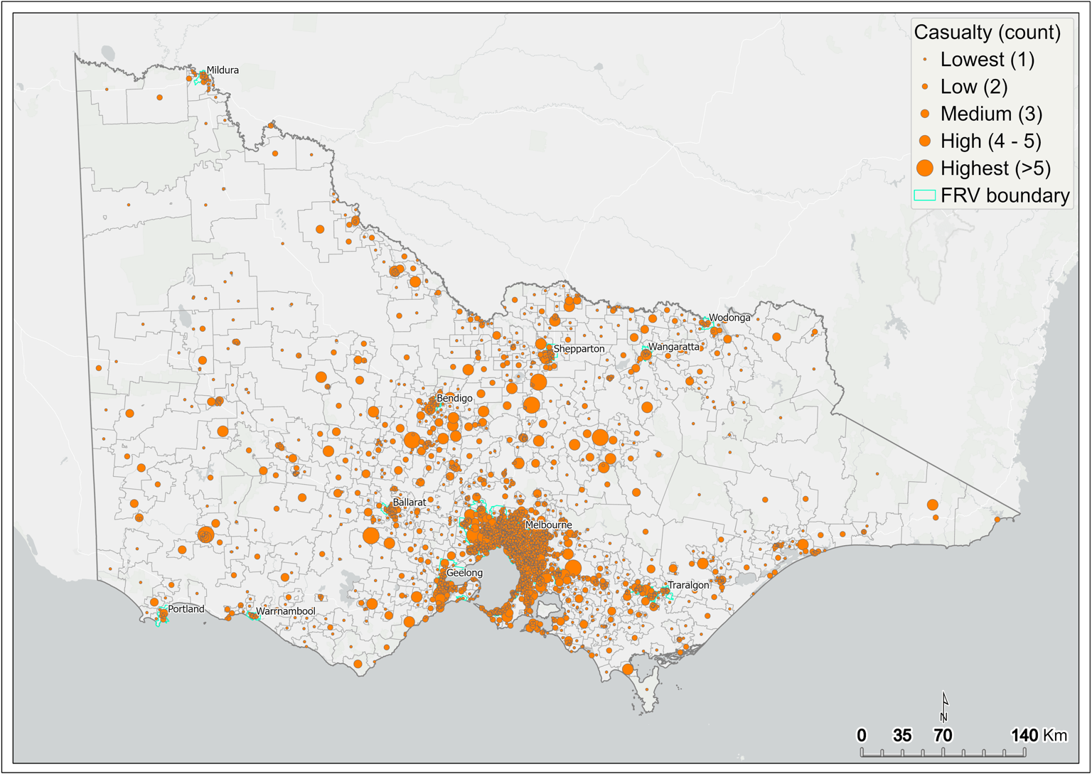
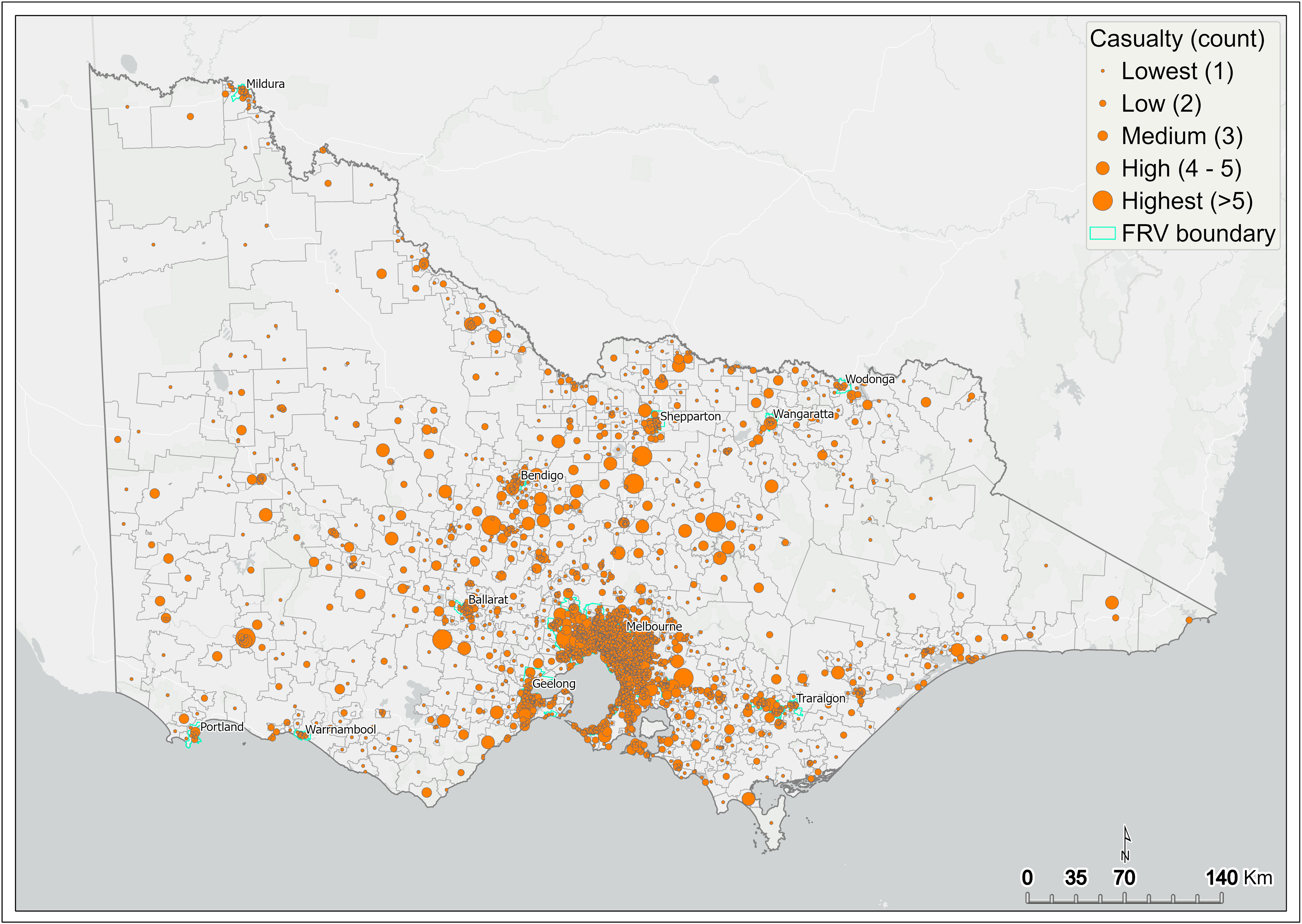
Cluster analysis is used to map the count of fire casualties (fatality and injury) across Victoria. Incidents resulting in casualties from 2010 to 2019 are mapped with graduated symbols showing a score from one to greater than five casualties per SA1. Figure 12 shows a map of the count of casualties resulting from fire incidents across SA1s of Victoria. The output from this analysis was subsequently input to the initial DSA.

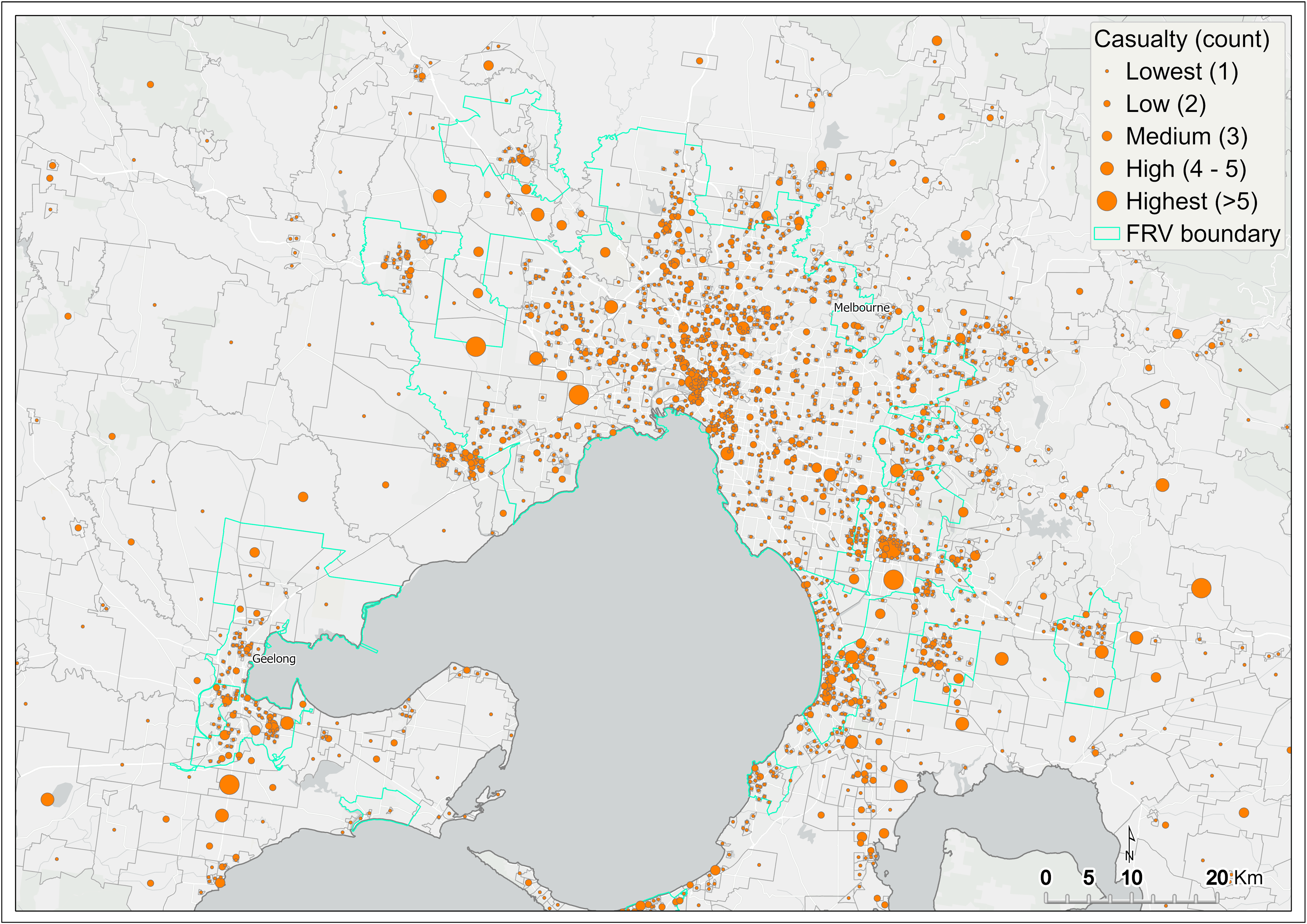
The greatest count of fire-related casualties is concentrated within metropolitan Melbourne (Figure 13). In the regions, fire-related casualty is high in central and northern parts of the Victoria. However, isolated regional centres in eastern and western Victoria demonstrate similarly high fire casualty count (Figure 12).

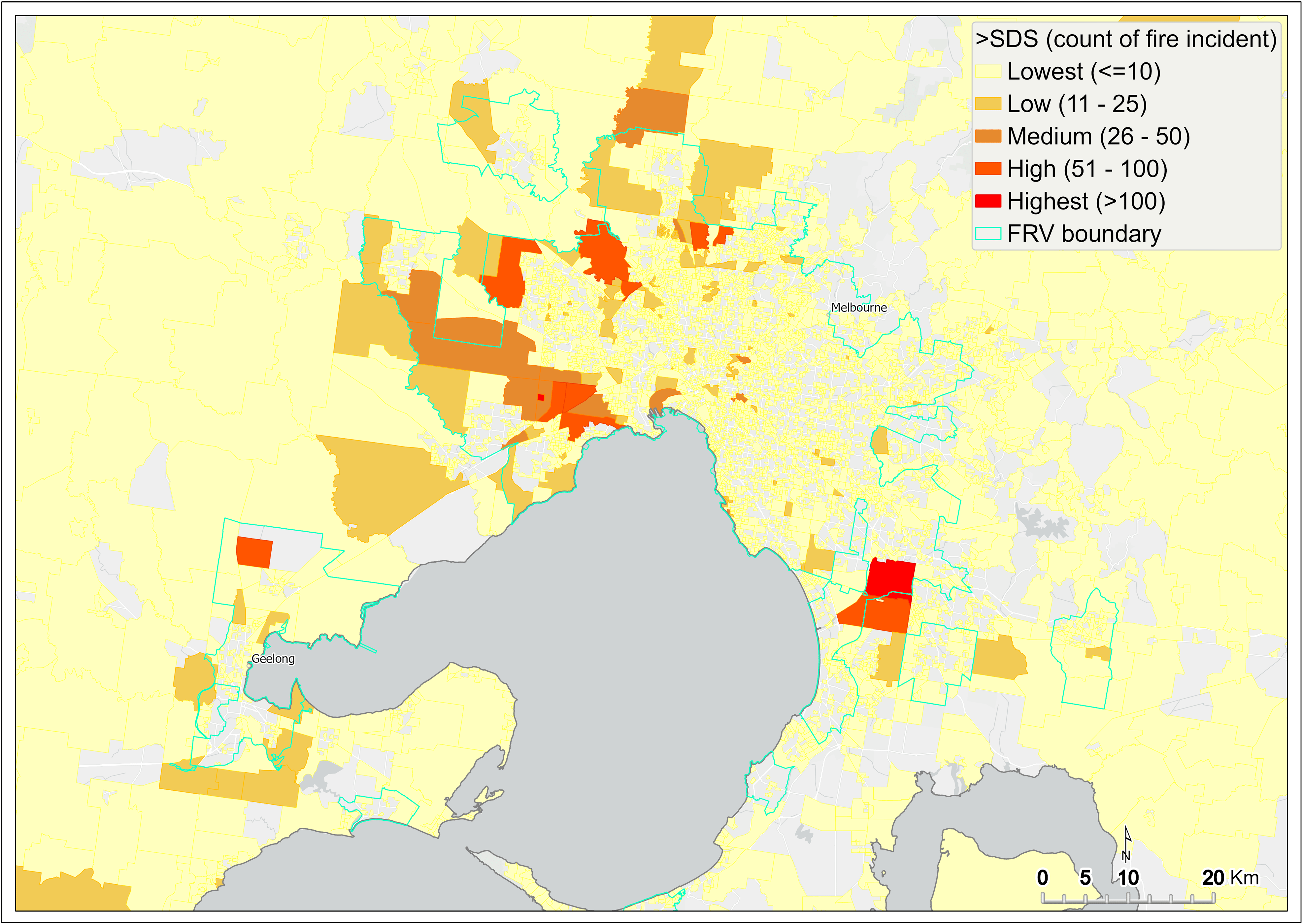
2.4.6 Service Delivery Standard failure mapping

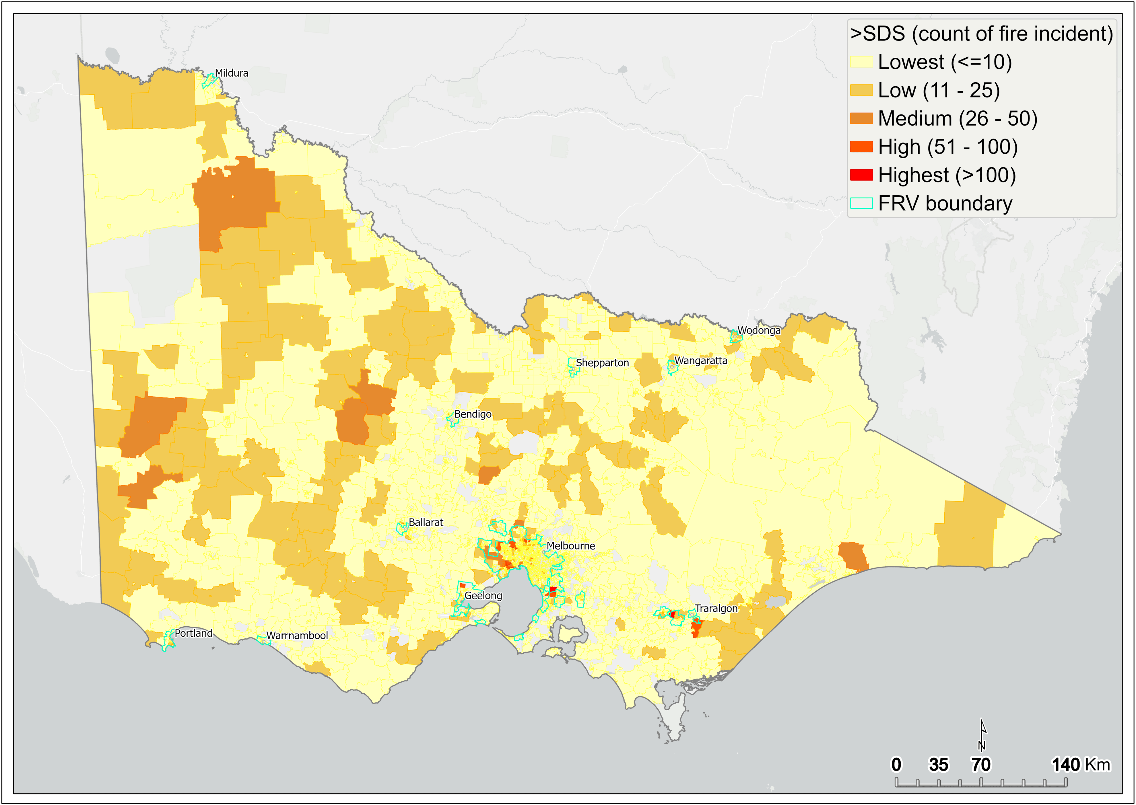
SDS⁴ (response time) failure is examined by mapping the count of fire incidents that failed to meet the SDS. The total count of incidents that failed to meet the SDS is categorised into five groups:

Lowest (≤10), Low (11 to 25), Medium (26 to 50), High (51 to 100) and Highest (>100).

Figure 14 shows a spatial pattern of the count of fire incidents that failed to meet the SDS statewide, and Figure 15 shows the same for metropolitan Melbourne. SA1s containing the lowest number of such incidents (that is, one to 10) not meeting the SDS are shown in yellow. These SA1s are located across much of regional Victoria and most parts of metropolitan Melbourne. SA1s containing zero incidents failing the SDS are not mapped.

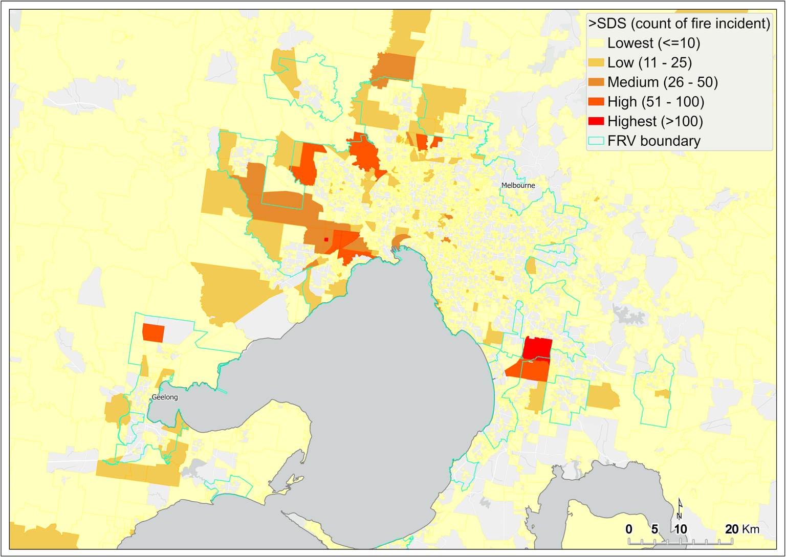
SDS failures have the potential to increase injury and fatality, so SA1s containing a high number of incidents not meeting the SDS are of major concern. The SA1s in the two highest categories (51 to 100 incidents and more than 100 incidents) are mainly located on the western metro fringe, straddling the FRV south-east boundary and in Gippsland. SA1s with greater than 100 incidents that were not responded to within SDS (highest category) are shown in red.

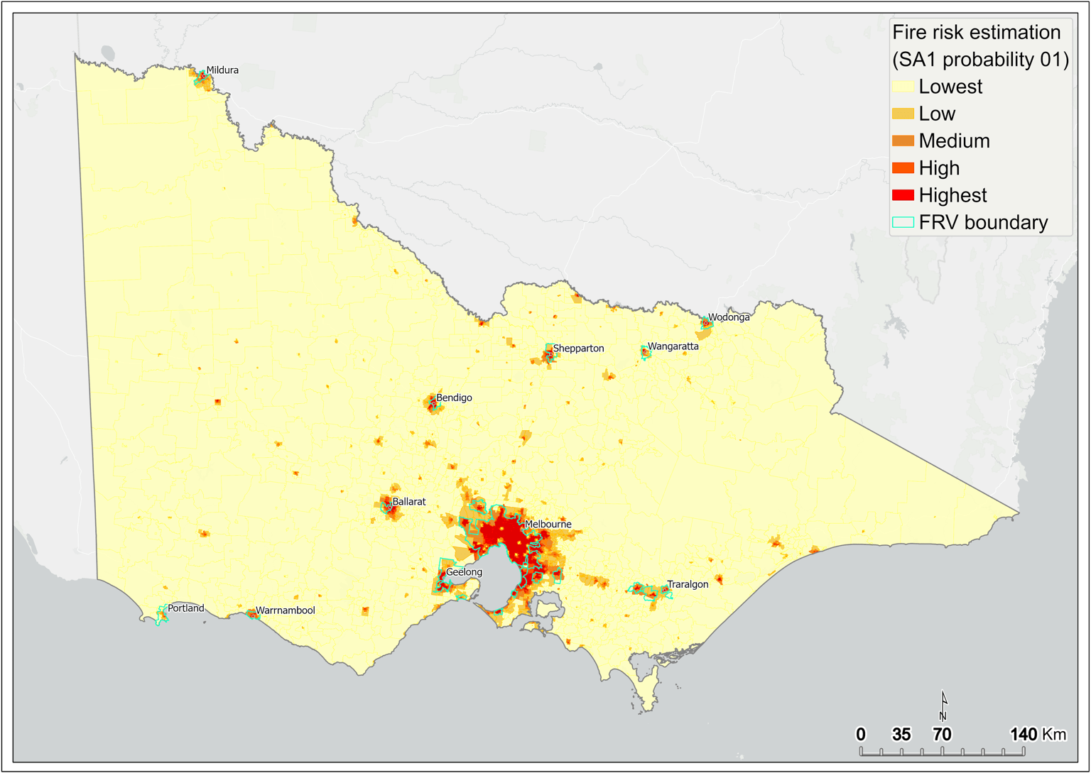
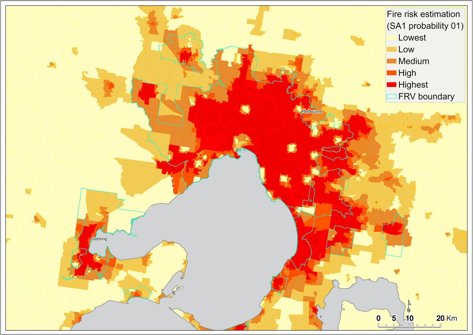
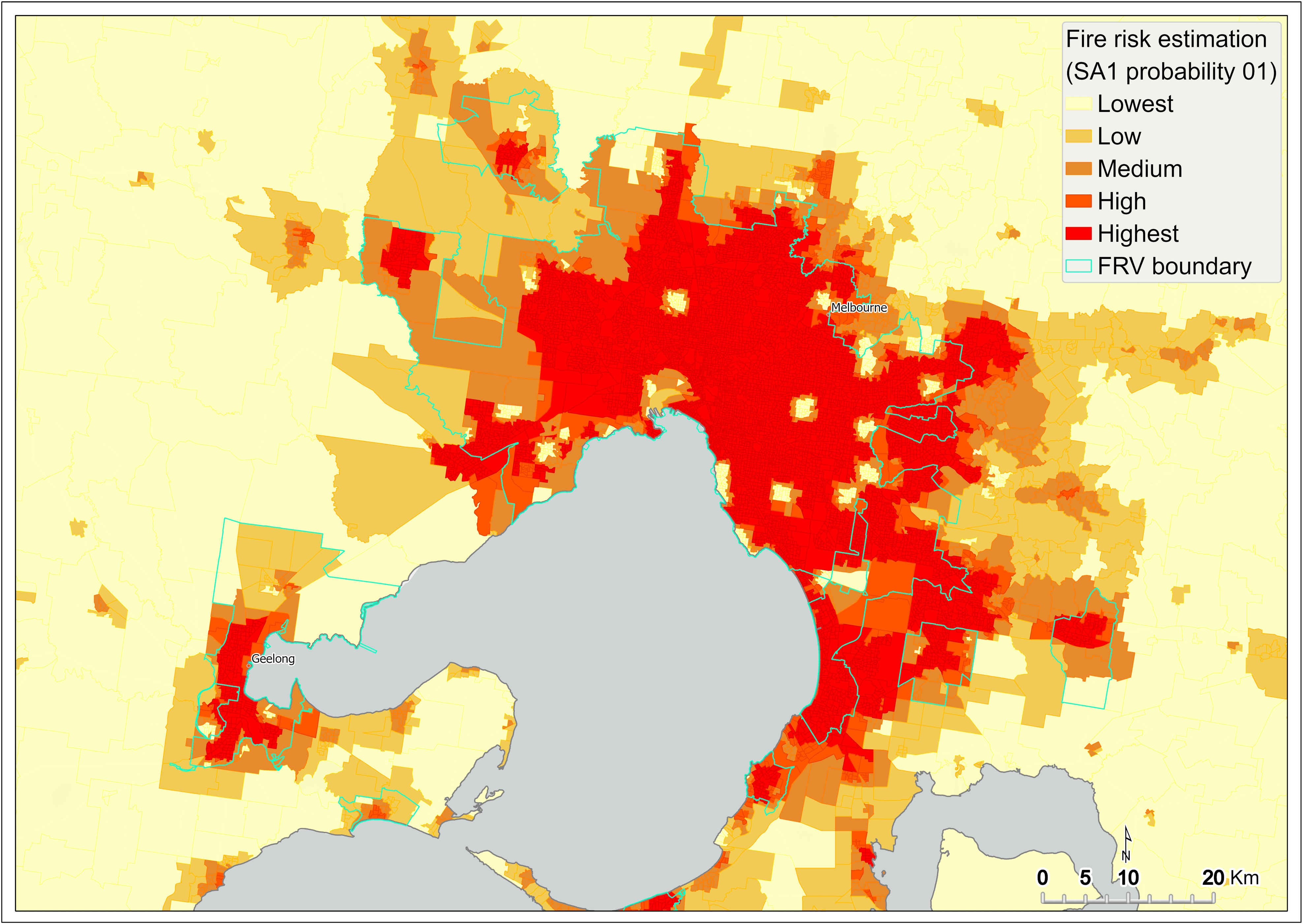
2.5 Fire risk estimation

Fire risk is estimated using two-step Markov chain⁵ modelling. The Markov chain estimation (MCE) routine is run across a statewide grid. The grid cells facilitate the transition from one scenario to another. A single transition is referred to as a step. Our analysis is two-step, which investigates the transition from no fire to fire (P01).

P01 =
the probability of fire in grid at t given no fire within neighbourhood at t-1

The results from this modelling are subsequently aggregated to the SA1 scale. The estimated probability of having at least one fire at time (t) given there was no fire in within the neighbourhood in past (t-1) is categorised into five groups:

Lowest (≤10%), Low (>10% to ≤25%), Medium (>25% to ≤50%), High (>50% to ≤75%) and Highest (>75%).

The areas of the state having greater than 50 per cent of probability of fire risk are predominantly concentrated within metropolitan Melbourne (Figure 17), as well as some regional centres such as greater Ballarat, Bendigo, Shepparton, Wodonga and around Traralgon (Figure 16).

Footnotes

[2] Involving two variables

[3] Statistical significance helps quantify whether a result is likely due to chance or to some factor of interest.

[4] Incidents coded as ‘excluded from SDS’ were not included in this analysis.

[5] https://towardsdatascience.com/introduction-to-markov-chains-50da3645a50d